Z-MR (Standardized Short Run) Chart
The Z-MR chart is a SPC Chart PRO short-run chart — it lets many different parts share a single control chart when no one part runs long enough to chart on its own.
Short production runs are a common problem for control charting: a job shop or a flexible line might make a few pieces of one part, switch to another, then another, and collect too few observations of each part to establish a reliable separate baseline. Z-MR solves this by standardizing every measurement — subtracting the part's mean and dividing by a standard deviation estimated with the selected method — so that parts with different nominal sizes and different amounts of variation all plot on one common scale centered on zero.
When to Use It
Use Z-MR when you run short batches of different parts and the parts differ in how much they vary, not just in size. Pooling raw deviations from parts with different process variation can let the part with the largest spread dominate the chart. Select a sigma estimation method that matches how variation differs between parts or runs.
If every part varies by about the same amount, the simpler DNOM chart is the better choice — it plots deviations in the original measurement units, which are easier to read and to relate back to a tolerance. Z-MR trades those units for the ability to mix parts with unequal variation.
| Your parts | Chart |
|---|---|
| Different nominals, similar variation | DNOM |
| Different nominals and different variation | Z-MR |
How It Works
Your query returns one row per measurement with a column identifying the part. Consecutive rows of the same part form a run; a part may appear in several runs as the line switches back and forth.
Each measurement is standardized against its own part:
zᵢ = (xᵢ − μ̂part) / σ̂
where μ̂part is the mean of every observation of that part, pooled across all of its runs, and σ̂ is the standard deviation estimate at the scope of the sigma method you choose.
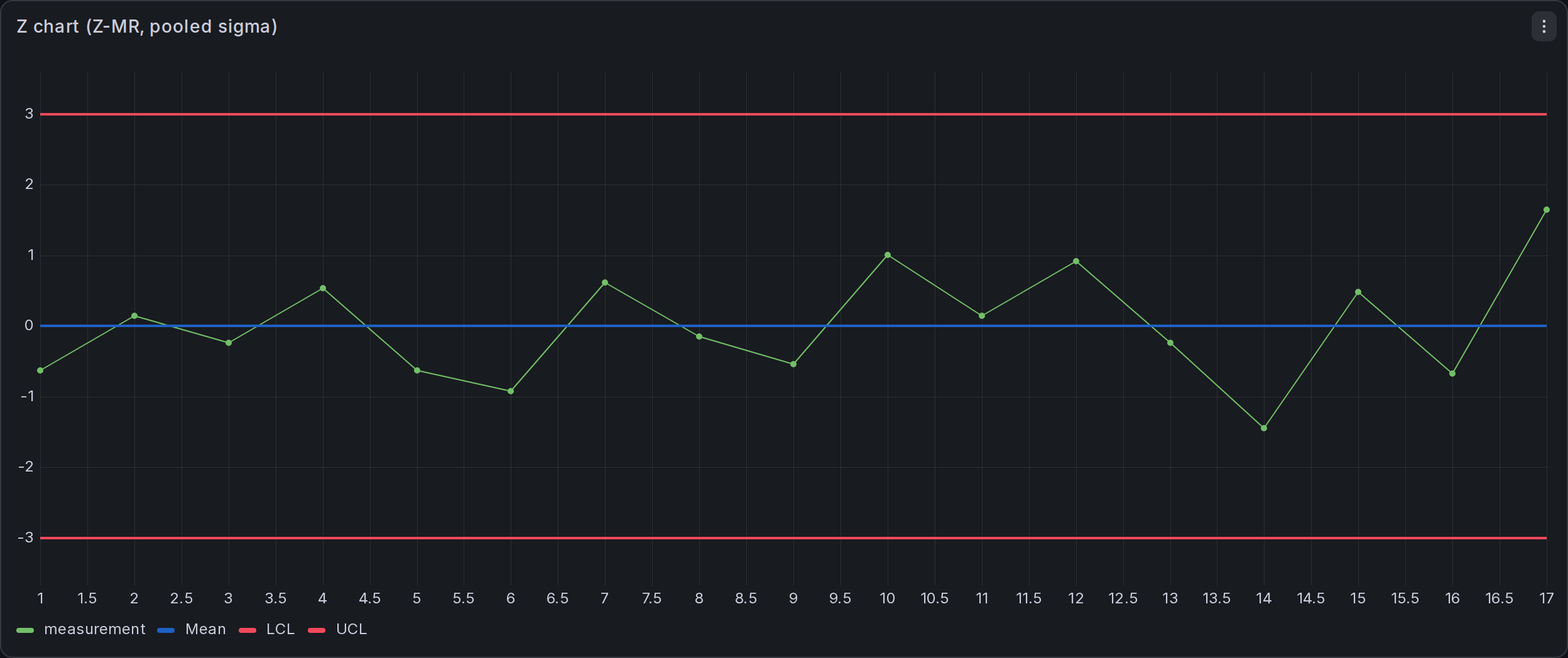
Because a z value is measured in standard deviations, the Z chart uses a center line of 0 and fixed limits at ±3. The companion MR chart has its own fixed limits, listed below. Requeries can still change the plotted values when the estimated part means or sigma values change.
| Chart Type (in the dropdown) | Plots |
|---|---|
| Z chart (Z-MR short run) | Each measurement standardized against its own part |
| MR chart (Z-MR short run) | The moving range of consecutive standardized values |
Moving ranges are computed within a run only; they never span a part changeover. A missing measurement or a blank part cell breaks the chain the same way.
Setting It Up
In the SPC section, with a Z-MR chart type selected:
| Option | Description |
|---|---|
| Part field | The field (text or number) that identifies each row's part. Consecutive rows of one part form a run. The field is hidden from the plot. |
| Sigma estimation | How the standard deviation used to standardize is estimated. See below. |
Standardized values are not plotted where sigma cannot be estimated or is zero. Each estimation pool needs at least one valid within-run moving range with nonzero average range.
Add a Z panel for the standardized values and an MR panel for the within-run spread, both pointing at the same query with the same Part field and Sigma estimation.
Sigma Estimation Methods
All four methods estimate sigma from average moving ranges within runs (MR̄ / d₂); they differ in how widely those ranges are pooled before the division. The methods follow Minitab's Z-MR estimation options.
| Method | Estimation scope | Use when |
|---|---|---|
| Constant (pool all data) | Once, from the moving ranges of every run on the chart | The parts share a common variance. This is the default and uses all available within-run moving ranges. |
| Relative to size (ln transform) | Once, on log-transformed measurements | Variation grows in proportion to the measurement — a 200 mm feature varying ten times as much as a 20 mm one. |
| By parts (combine runs of a part) | Per part, from the moving ranges of all that part's runs | Each part has its own variation, and a part's behavior is stable across the runs it appears in. |
| By runs (each run independently) | Per run, from that run's own moving ranges | Even the same part varies differently from run to run — a new machine setup between runs, for example. Needs the most data per run. |
Choose Constant when the parts share a common variance, or Relative to size when variation scales with measurement size. By parts and By runs estimate sigma from smaller pools of data and therefore require enough observations in each pool. For example, a run of four measurements provides only three moving ranges.
Relative to size takes the natural log of each measurement first, so it needs strictly positive values. Both the part means and moving ranges are calculated on the log-transformed data. Rows with a zero or negative measurement cannot be transformed and are treated as gaps.
Methods and Formulas
Let μ̂part be the mean of all valid observations of a part and MR̄ the average moving range within runs at the scope of the chosen method. For Relative to size, xᵢ denotes ln(measurementᵢ), and both estimates use that transformed scale.
| Quantity | Formula |
|---|---|
| Sigma estimate | σ̂ = MR̄ / d₂ = MR̄ / 1.128 |
| Standardized value | zᵢ = (xᵢ − μ̂part) / σ̂ |
| Chart | Center line | Control limits |
|---|---|---|
| Z (standardized values) | 0 | +3 and −3 |
| MR (of z values) | d₂ = 1.128 | D₂ = 3.686 and 0 |
The Z chart uses the reference scale σ = 1 after standardization; the observed sample standard deviation need not equal exactly 1. For the same reason the MR chart uses the known-sigma constants for a moving range of two — d₂ and D₂ applied to σ = 1 — rather than deriving its limits from the plotted ranges the way an ordinary mR chart does.
The part column is read as an input and hidden from the plot. Capability indices are not shown for short-run charts, since the chart pools several parts, and the Control limits section does not apply — Z-MR has its own Sigma estimation option instead. The part field, sigma method, and chart type are saved with the dashboard, and the chart works with both a time and a numeric X-axis.
Z-MR is part of SPC Chart PRO. See requirements, licensing, and support.