SPC CAD
The SPC CAD Panel brings 3D geometry into Grafana, letting you visualize CAD models, point clouds, and metrology data alongside live measurements — so you can see quality data in the context of the actual part geometry.
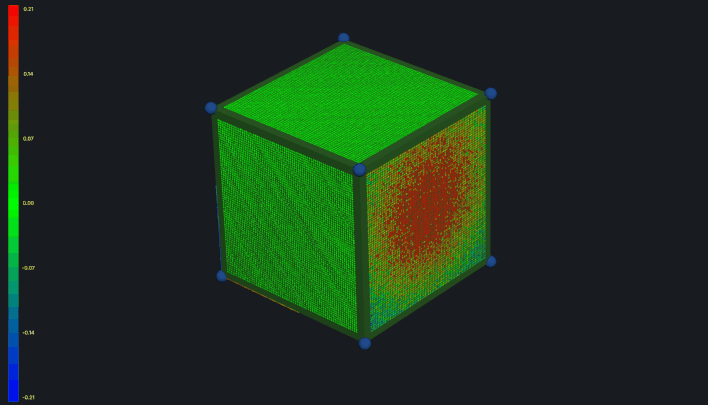
Table of Contents
- Why SPC CAD?
- Built for Grafana
- Features
- Use Cases
- Requirements
- Getting Started
- Supported File Formats
- Data Model Requirements
- Features and Characteristics
- CAD Model Configuration
- Annotations System
- Annotation Editor
- Templates
- Color Mapping
- Forecasting
- Point Clouds
- Panel Options
- 3D Navigation
- Advanced Topics
- Troubleshooting
- Part of the KensoBI SPC Suite
- Getting Help
- License
Why SPC CAD?
Quality data makes more sense when you can see it on the actual part. The SPC CAD Panel bridges the gap between dimensional metrology and 3D visualization:
- Context for measurements — see exactly where each feature is located on the part geometry
- Interactive annotations — click any feature to view detailed measurement data, control charts, and historical trends
- Conditional color coding — instantly identify out-of-spec features with visual alerts based on measurement rules
- Point cloud integration — overlay scan data with deviation coloring to spot problem areas at a glance
- Live data binding — annotations update automatically as new measurements arrive from your data source
Built for Grafana
SPC CAD is built using Grafana's native panel framework and follows Grafana's design patterns:
- Native theming — automatically adapts to light and dark mode
- Dashboard integration — works seamlessly with time ranges and data sources
- Standard panel options — familiar configuration interface just like any other Grafana panel
- Works with any data source — use it with SQL databases, time series databases, or custom data sources that return metrology data
Features
| Feature | Description |
|---|---|
| 3D CAD models | Display STL, 3MF, PLY, and image files with full 3D navigation |
| Point cloud visualization | Load ASC and PLY scan data with deviation-based color gradients |
| Interactive annotations | Click features to view measurement data, charts, and statistics |
| Customizable templates | 13 built-in templates for common metrology features (point, circle, cylinder, etc.) |
| Color mapping | Conditional styling based on measurement rules (pass/fail, tolerance zones) |
| Time series charts | Embed SPC control charts and trend analysis in feature annotations |
| Multiple data views | Tables, grids, and charts in tabbed annotation layouts |
| URL linking | Deep link to ERP, MES, or CMM systems with variable substitution |
| Forecasting support | Display prediction trends with confidence bands |
| Scan timeline | Navigate through historical point cloud data with playback controls |
| Dynamic positioning | Auto-position features from X, Y, Z characteristics or place manually |
| Dashboard variables | Use Grafana variables in model URLs and link templates |
Use Cases
- Manufacturing quality — visualize CMM inspection results on part geometry
- Production monitoring — track dimensional trends on critical features over time
- First article inspection — create interactive 3D inspection reports
- Root cause analysis — correlate out-of-spec features with process parameters
- Supplier quality — compare scan data against nominal geometry to identify deviations
- Process validation — verify that parts meet specification across production runs
- Metrology reporting — generate visual quality reports for stakeholders
Requirements
- Grafana 11 or later
Getting Started
- Install the SPC CAD plugin from the Grafana Plugin Catalog
- Create a new panel and select SPC CAD as the visualization type
- Add a CAD model using the panel options (from URL or upload a file)
- Configure a data source query that returns feature and characteristic data
- Click on features in the 3D view to create interactive annotations
Quick Example:
To create a basic CAD visualization with positioned features:
- In panel options, add a CAD model URL:
https://example.com/model.stl - Configure a query that returns:
feature— Feature name (string)characteristic_id— Unique identifier (string)nominal— Nominal value (number)- X, Y, Z characteristics for automatic positioning
- Features will appear on the model at their X, Y, Z coordinates
- Click any feature to open an annotation with measurement data
For detailed data requirements, see Data Model Requirements.
Supported File Formats
The panel supports multiple file formats for both CAD models and point clouds:
CAD Models
| Format | Extension | Description | Use Case |
|---|---|---|---|
| STL | .stl | Stereolithography (binary/ASCII) | Most common 3D model format |
| 3MF | .3mf | 3D Manufacturing Format | Modern alternative to STL with color support |
| PLY | .ply | Polygon File Format | Point clouds and meshes with custom attributes |
| ASC | .asc | ASCII Point Cloud | Deviation/comparison data |
| Images | .jpg, .png, .svg | 2D images | Technical drawings or reference images |
Compression Support: All formats can be GZIP compressed (.gz, .gzip extensions)
Recommended file size: Up to 200 MB (5 MB limit for uploads)
ASC Deviation File Format
ASC files are used for point cloud deviation data. Each line represents a measurement point with space-separated values:
Name X Y Z Nx Ny Nz DevX DevY DevZ DevTotal
Name- String identifier for the surface comparisonX Y Z- Coordinates of the measurement pointNx Ny Nz- Surface normal vector componentsDevX DevY DevZ- Deviation components along each axisDevTotal- Absolute magnitude of total deviation
Example:
Surface_comparison_cube 5.000000 5.000000 0.000000 0.000000 0.000000 -1.000000 -0.000000 -0.000000 0.080942 0.080942
All numeric values should be floating-point with six decimal places. No header row is required.
Data Model Requirements
The panel expects data in a specific structure from your Grafana queries. Understanding this structure is crucial for proper visualization.
Required DataFrame: Features
Your primary query should return feature and characteristic data:
Required Columns
feature- Feature name/identifier (string)characteristic_id- Unique identifier for each characteristic (string or number)characteristic_name- Display name for the characteristic (defaults to characteristic_id)nominal- Nominal/reference value (number)
Optional But Recommended Columns
partid- Part identifier for groupingfeaturetype- Feature type classification (point, circle, cylinder, etc.)
Additional Columns
Any additional columns in your query will be treated as characteristic data fields and will be available for display in annotations, tables, and color mapping rules.
Example Query Result:
| feature | characteristic_id | nominal | characteristic_name | x | y | z | measured | tolerance |
|---|---|---|---|---|---|---|---|---|
| Hole_01 | char_001 | 10.0 | X Position | 10.0 | 0 | 0 | 10.05 | 0.1 |
| Hole_01 | char_002 | 20.0 | Y Position | 0 | 20.0 | 0 | 19.98 | 0.1 |
| Hole_01 | char_003 | 5.0 | Z Position | 0 | 0 | 5.0 | 5.02 | 0.1 |
| Hole_01 | char_004 | 6.5 | Diameter | 0 | 0 | 0 | 6.48 | 0.05 |
Optional DataFrame: CAD Models
You can load CAD models from your data source by returning a DataFrame with:
links- URL or path to CAD filecolors- Hex color code for the model (e.g.,#FF0000)
Optional DataFrame: Scan Timeline
For time-series point cloud data, create a DataFrame named scans:
links- URL to scan filetimes- Timestamp of the scan (Grafana time format)
This enables the scan timeline slider for navigating through historical scan data.
Optional: Time Series Data
To display charts in annotations, include time-series data in either:
- Grafana Time Series Format - Standard Grafana time field with value columns
- Long Format with columns:
time- Timestampcharacteristic_id- Characteristic identifiervalue- Measurement value
The panel will automatically filter null values and associate time series data with characteristics.
Features and Characteristics
In dimensional metrology, a feature refers to a specific geometric element of a component being measured (e.g., hole, surface, edge). Each feature consists of one or more characteristics - measurable properties like position, diameter, angle, or surface finish.
Feature Positioning
Features are positioned in 3D space when they have X, Y, and Z characteristics with valid nominal values. The panel looks for characteristics named:
X,x, or characteristic names containing "X Position"Y,y, or characteristic names containing "Y Position"Z,z, or characteristic names containing "Z Position"
Position Resolution Modes:
- Automatic - X, Y, Z characteristics found with valid nominal values
- Custom - Manually positioned using the unpositioned features editor
- No Position - Feature explicitly marked as having no position (annotation-only)
- Undefined - No position data available (must be manually positioned)
Working with Unpositioned Features
If features lack position data, they appear in the Unpositioned Features Editor in panel options:
- Select a feature from the list
- Click "Position Feature" to enter placement mode
- Click anywhere on the 3D scene to place the feature
- Save or cancel the positioning
Alternatively, features can be used without 3D positioning - annotations will appear in window mode without a 3D marker.
CAD Model Configuration
Adding Models from URL
- Open panel options and navigate to "CAD Models"
- Click "Add CAD Model"
- Enter the URL to your model file
- (Optional) Choose a custom color for the model
- Save the panel
Example URLs:
https://example.com/models/part.stl/public/models/housing.3mf${variable}/path/to/model.stl(with dashboard variables)
Uploading Models
For local files or testing:
- Click "Upload File" in the CAD models section
- Select a file (max 5 MB)
- The file will be embedded as Base64 data in the panel configuration
Note: Uploaded files increase panel configuration size. For production, prefer hosting files separately and using URLs.
Model Appearance
Each model can be customized:
- Color - Click the color picker to change the model's color
- Visibility - Toggle models on/off
- Multiple Models - Add multiple models to the same scene
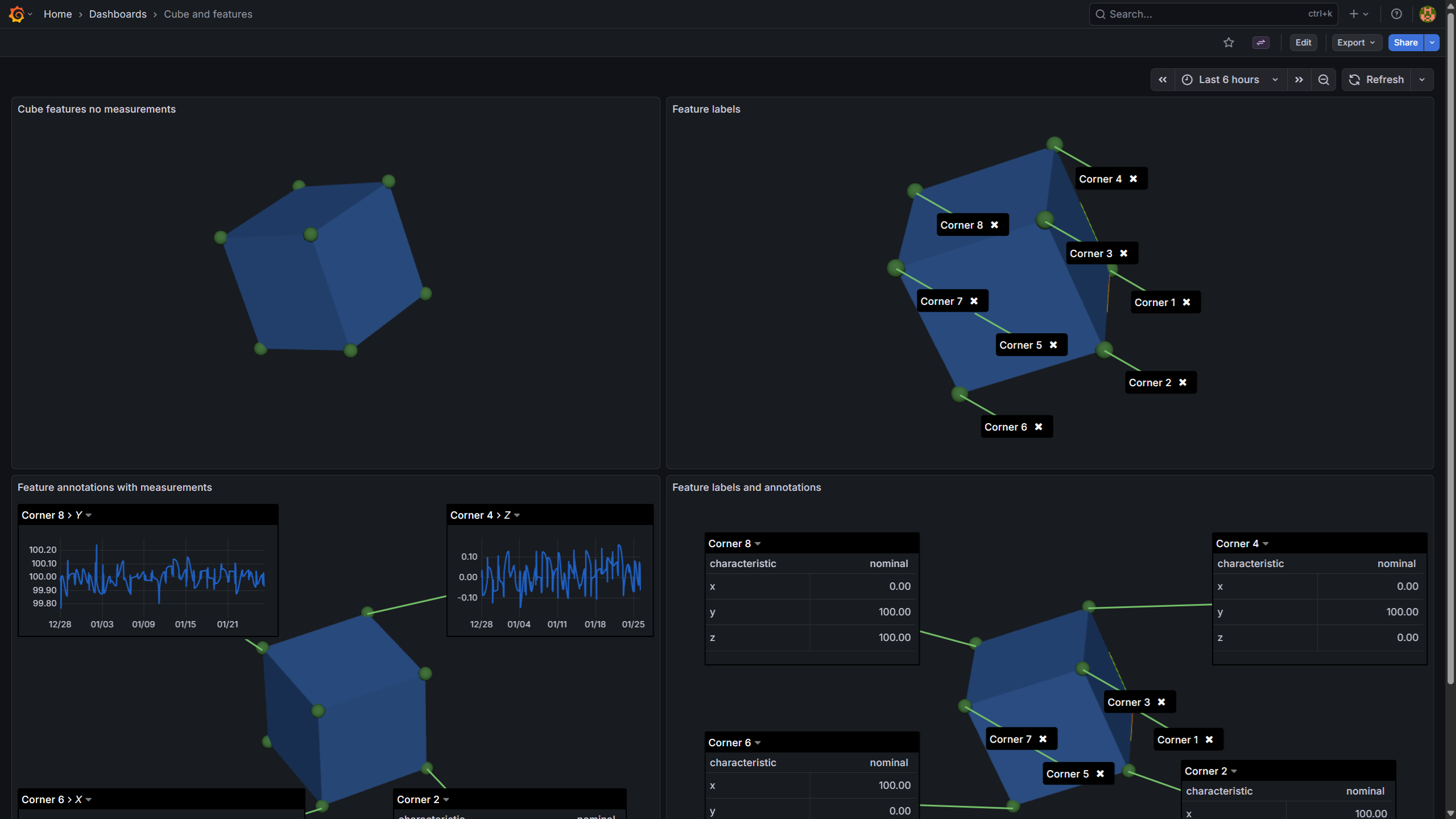
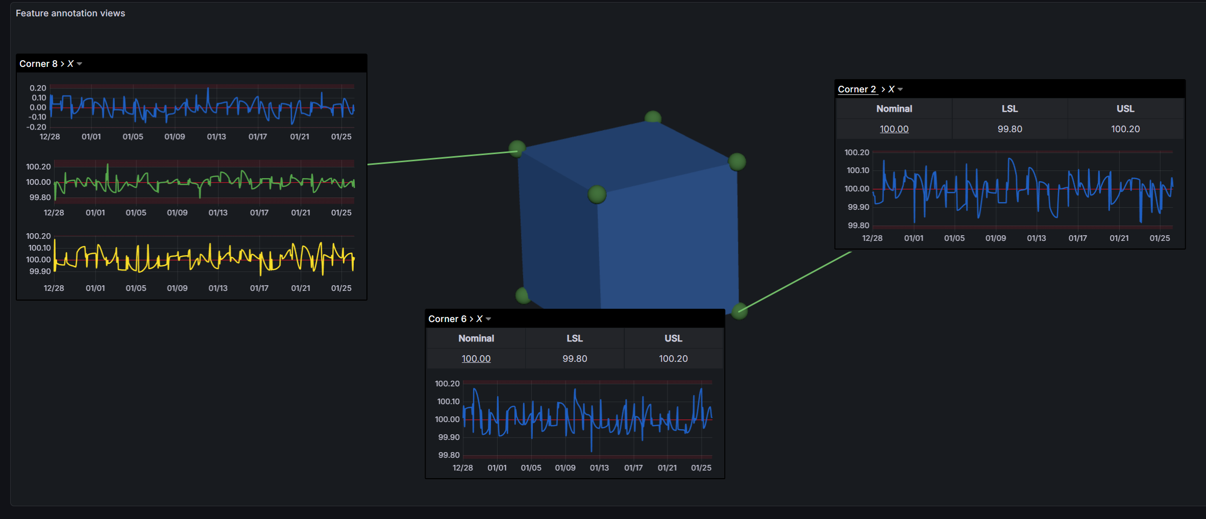
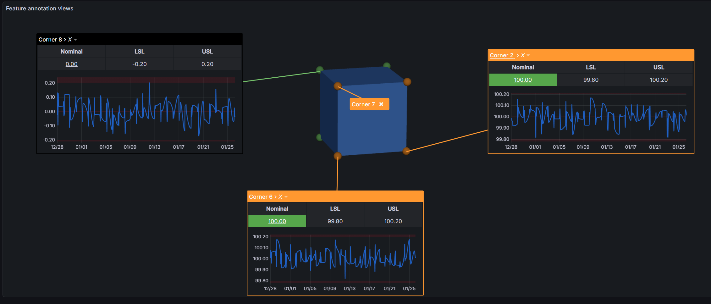
Annotations System
Annotations are interactive information boxes that display data about features. They consist of a 3D label/marker and an expandable window containing customizable views.
Annotation Display Modes
Each annotation has three display states:
- Hidden - Annotation not visible
- Label - Compact floating label that follows the feature
- Shows feature title
- Can be colored based on data values
- Click to expand to window mode
- Window - Fixed panel with full content
- Resizable and draggable
- Contains multiple views/tabs
- Grid layout positioning
Creating Annotations
- Click on a feature in the 3D view
- An annotation is automatically created in label mode
- Click the label to expand it to a window
- Use the pin icon to keep the window open
Annotation Settings
Each annotation can be configured independently:
- Title Column - Choose which data column to display as the title
- Template - Select a template for the annotation layout (see Templates)
- Color Rules - Apply conditional styling to the header (see Color Mapping)
- Link - Add URL linking with variable substitution
- Grid Position - Manually position and resize windows
Annotation Editor
The Annotation Editor provides full customization of annotation content and appearance.
Accessing the Editor
Two ways to open the editor:
- Double-click on any annotation view
- Click the gear icon in the annotation header
View System
Annotations support multiple views (tabs), each containing one or more components. Views can be:
- Added, removed, and reordered
- Named for easy navigation
- Set as the default active view
Component Types
1. Table Component
Displays characteristic data in tabular format.
Configuration:
- Columns Filter - Show only specific columns (leave empty for all)
- Rows Filter - Show only specific characteristics (leave empty for all)
- Decimals - Number of decimal places (default: 2)
Features:
- Automatically displays all available columns across characteristics
- Row headers show characteristic names
- Values retrieved from the data query
Use Cases:
- Showing all measurements for a feature
- Comparing nominal vs. actual values
- Displaying tolerance information
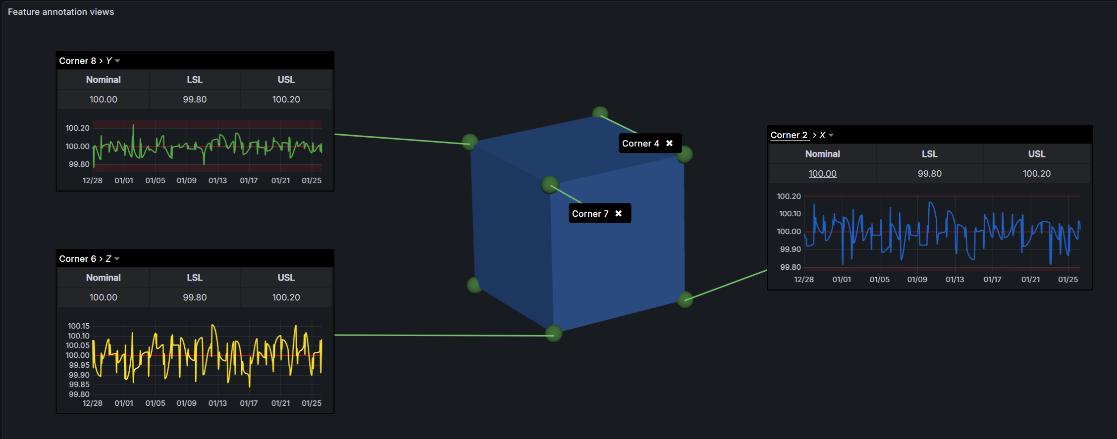
2. Time Series Component
Displays measurement trends over time using line/area charts.
Configuration:
- Characteristic - Select which characteristic to plot
- Line Color - Customize the line color (default: blue)
- Line Width - Line thickness in pixels (default: 2)
- Fill - Area fill percentage 0-100 (default: 0)
- Point Size - Data point marker size (default: 6)
- Show Legend - Display legend (default: false)
- Decimals - Y-axis number formatting (default: 2)
Advanced Options:
- Limit Lines - Add upper and lower specification limits
- Constant Lines - Add reference lines with custom colors
- SPC Integration - Statistical process control chart support
Use Cases:
- Trending measurements over time
- Control chart visualization
- Process stability monitoring
3. Grid Component
Flexible card-style layout for custom data presentation.
Configuration:
- Show Headers - Display column headers
- Grid Cells - Define individual cells with:
- Name - Cell label
- Value - Static text or dynamic data reference
- Color Mapping - Conditional styling per cell
- Link - URL with variable substitution
- Suffix - Append units or text
- Decimals - Number formatting
Features:
- Fully customizable layout
- Per-cell conditional formatting
- Static and dynamic content mixing
- URL linking with context
Use Cases:
- Dashboard-style summary cards
- Key metrics display
- Pass/fail indicators with color coding
Creating Custom Views
- Click "Add View" in the annotation editor
- Choose a view name
- Add components:
- Click "Add Table", "Add Time Series", or "Add Grid"
- Configure each component's settings
- Reorder components by dragging
- Save the annotation
Drag and Drop
Components within a view can be reordered by dragging. This allows you to arrange information in the most logical order for your workflow.
Templates
Templates are predefined annotation layouts for different feature types. The panel includes 13 built-in templates, each optimized for specific geometric features.
Built-in Templates
- Generic (Default) - Multi-view layout with Main, X, Y, Z tabs
- Point - Single point feature
- Circle - Circular features (holes, pins)
- Cylinder - Cylindrical features
- Sphere - Spherical features
- Ellipse - Elliptical features
- Line - Linear features (edges)
- Rectangle - Rectangular features
- Slot - Slot features
- Plane - Planar surfaces
- Slab - Slab/block features
- Cone - Conical features
- Comparison Point - Point cloud comparison data
Using Templates
Automatic Template Selection:
If your data includes a featuretype column, the panel can automatically assign the appropriate template based on the feature type value.
Manual Template Assignment:
- Click on a feature to create an annotation
- Open the annotation editor (gear icon)
- Select a template from the dropdown
- The annotation layout updates immediately
Template System Benefits
Templates provide:
- Consistency - All features of the same type look identical
- Efficiency - No need to manually configure each annotation
- Best Practices - Pre-configured views for common metrology features
- Customization - Templates serve as starting points and can be overridden
Template Customization
While templates provide defaults, any annotation can be customized:
- Select a template
- Modify views, components, or settings
- The changes override the template for that annotation only
- Other annotations using the same template remain unchanged
Color Mapping
Color mapping allows you to apply conditional styling to annotations based on measurement data. This provides instant visual feedback on feature quality.
How Color Mapping Works
Color rules are evaluated top-to-bottom. The first matching rule determines the header color.
Color Rule Components:
- Left Side - Characteristic + column to evaluate
- Operator - Comparison type
- Right Side - Value or column to compare against
- Colors - Background and text color to apply
Supported Operators
<- Less than=- Equals>- Greater than
Mapping Types
Static Value Comparison
Compare a characteristic column against a fixed value.
Example: Highlight features where measured value exceeds nominal by more than tolerance
characteristic: "X Position"
column: "measured"
operator: >
value: 10.1
backgroundColor: #FF0000
textColor: #FFFFFF
Dynamic Column Comparison
Compare two columns within the same characteristic.
Example: Highlight when measured value deviates from nominal
characteristic: "Diameter"
column: "deviation"
operator: >
rightColumn: "tolerance"
backgroundColor: #FFA500
textColor: #000000
Configuring Color Rules
Template-Level Rules:
- Open panel options
- Navigate to "Templates"
- Select a template
- Add color rules
- Rules apply to all annotations using this template
Annotation-Level Rules:
- Open annotation editor
- Go to "Header Colors" section
- Add rules specific to this annotation
- Annotation rules override template rules
Color Rule Priority
- Annotation-specific rules (highest priority)
- Template-default rules
- Default annotation color (no rules matched)
Color Mapping Best Practices
- Use consistent color schemes across templates (e.g., green = good, yellow = warning, red = fail)
- Order rules from most specific to least specific
- Test rules with representative data before deployment
- Document your color coding in dashboard descriptions or annotations
Example: Pass/Fail Color Coding
Rule 1: deviation < -tolerance → Red background (below spec)
Rule 2: deviation > tolerance → Red background (above spec)
Rule 3: deviation between -tolerance and tolerance → Green background (pass)
Forecasting
The SPC CAD Panel can display forecast trends with confidence bands directly on feature time-series charts, helping you anticipate process drift before it leads to out-of-spec parts.
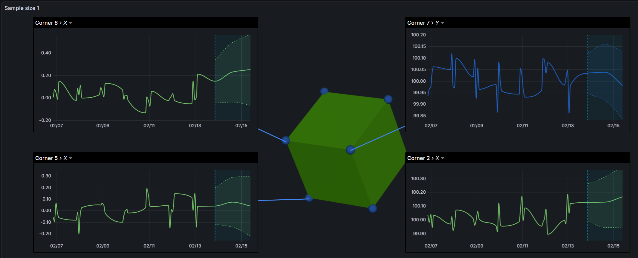
How It Works
The panel does not calculate forecasts itself. Forecast data is provided by a compatible datasource — such as the KensoBI SPC Characteristic Datasource — which returns forecast values along with upper and lower confidence bounds.
When forecast data is present in the query results, the time-series component automatically renders:
- Forecast line — the predicted trend extending beyond the last measured value
- Confidence band — a filled region between the upper and lower bounds, showing the range of expected variation
Requirements
To display forecasts in annotation charts:
- Use a datasource that returns forecast data (e.g., KensoBI SPC Characteristic Datasource)
- Add a time-series component to your annotation view
- The forecast region and confidence bands render automatically when forecast data is available
Use Cases
- Early warning — spot trends heading toward specification limits before they arrive
- Process planning — predict when tooling adjustments or maintenance will be needed
- Quality reporting — show stakeholders not just where you are, but where the process is heading
Point Clouds
Point cloud visualization is a powerful feature for displaying scan data and deviation analysis.
Loading Point Clouds
Point clouds can be loaded from:
- ASC files - Deviation data with point-by-point comparison
- PLY files - Generic point cloud format with optional deviation attributes
Via URL:
Add CAD Model → Enter ASC/PLY file URL
Via Data Query:
SELECT
  '/path/to/scan.asc' as links,
  '#FF0000' as colors
Deviation Visualization
When point clouds include deviation data, the panel automatically applies color gradient mapping:
- Blue - Negative deviation (below nominal)
- Green - Zero deviation (at nominal)
- Red - Positive deviation (above nominal)
The gradient is calculated based on standard deviation:
- Range = ±3σ (captures ~99.7% of points in normal distribution)
- 7-step gradient for smooth color transitions
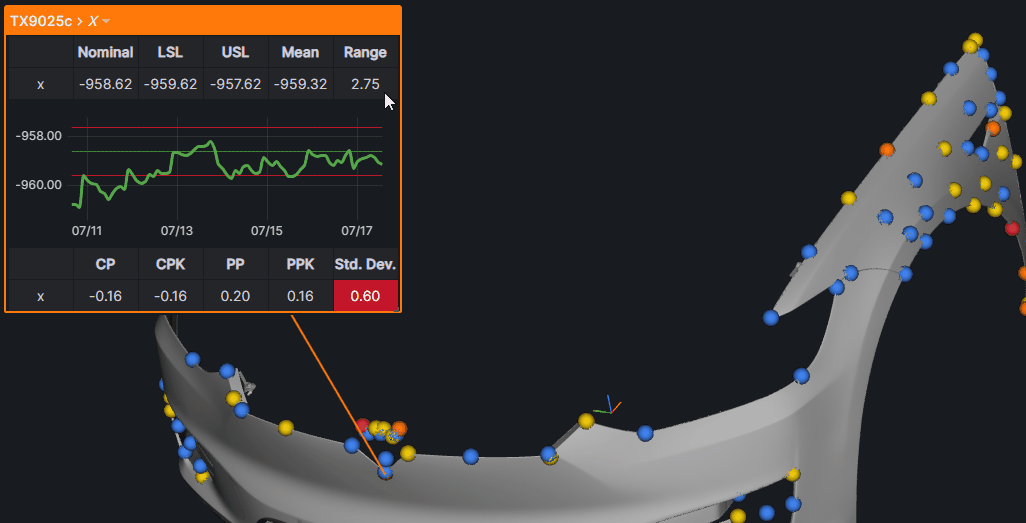
Gradient Legend
The gradient legend appears when a point cloud is loaded:
Features:
- Shows deviation range (min to max)
- Current hovered point value with crosshair indicator
- Automatic decimal precision based on range magnitude
- Standard deviation-based range calculation
Point Cloud Interaction
Hover over points to:
- See the deviation value in the legend
- Highlight the point with a red sphere marker
- View point coordinates
Benefits:
- Quickly identify problem areas
- Understand deviation patterns
- Compare actual vs. nominal geometry
Scan Timeline
For time-series point cloud data, use the scan timeline:
- Configure a
scansDataFrame in your query with:links- Scan file URLstimes- Timestamps
- A timeline slider appears at the bottom
- Use play/pause controls to animate through scans
- Click any point on the timeline to jump to that scan
Use Cases:
- Part inspection over time
- Process monitoring
- Historical comparison
- Quality trend analysis
Panel Options
The panel provides extensive configuration options organized into sections.
CAD Models Section
- Add Model - Add CAD models from URL
- Upload File - Upload local files (max 5 MB)
- Model Color - Customize model appearance
- Remove Model - Delete models from the scene
Feature Settings
- Feature Size - Control the size of feature markers (range: 1-200)
- Smaller values: More subtle markers
- Larger values: Easier to click, more prominent
- Default: 10
- Feature Color - Default color for features without color mapping
Scene Settings
- Camera Position - X, Y, Z coordinates (default: 0, 0, 2500)
- Camera Target - Look-at point X, Y, Z (default: 0, 0, 0)
- Camera Up Vector - Orientation (default: 0, 1, 0)
These settings persist when you refresh the dashboard, maintaining your viewing angle.
Annotation Settings
- Title Column - Default column for annotation titles
- Template - Default template for new annotations
- Pin by Default - Whether new annotations open as windows or labels
Unpositioned Features
- Feature List - Shows features without 3D position data
- Position Tool - Click-to-place positioning interface
- Manual Positioning - Enter exact X, Y, Z coordinates
3D Navigation
The panel uses intuitive trackball controls for 3D navigation.
Mouse Controls
- Left Click + Drag - Rotate the view around the target point
- Scroll Wheel - Zoom in/out
- Middle Click + Drag - Pan the view
- Right Click - Open feature context menu (when over a feature)
View Helper
A 3D orientation cube appears in the corner:
- Shows current view orientation (X, Y, Z axes)
- Click any face to snap to that view
- Helps maintain orientation in complex scenes
Camera Presets
While the panel doesn't include built-in view presets, you can:
- Position the camera as desired
- The position is saved in panel options
- Export/import panel JSON to save views
- Use dashboard variables to switch between camera positions
Navigation Tips
- Start with a top-down view (Z-axis) for 2D-like inspection
- Use pan to center features of interest before rotating
- Zoom in on small features before attempting to click them
- Reset view by entering default camera settings in panel options
Advanced Topics
URL Linking
Both annotations and grid cells support dynamic URL linking:
Variable Substitution:
- Use
${fieldName}to insert data values - Example:
https://erp.example.com/parts/${partid}
Configuration:
- URL template with variables
- Open in new tab option
- Available in:
- Annotation-level settings
- Grid cell settings
Dashboard Variables Integration
The panel supports Grafana dashboard variables in:
- CAD model URLs
- Link URLs
- Panel titles
Example:
Model URL: /models/${partNumber}.stl
Link URL: https://mes.example.com/${line}/${batch}
Multi-Part Assemblies
To display multiple parts simultaneously:
- Load multiple CAD models
- Use
partidcolumn in your data to associate features with specific models - Color code models by part for easy identification
- Position models relative to each other using coordinate offsets
Performance Optimization
For Large Models:
- Use compressed files (
.gz) - Prefer binary STL over ASCII STL
- Consider decimating meshes before loading
For Many Features:
- Reduce feature size if many overlap
- Use label mode instead of window mode by default
- Filter data to show only relevant features
For Time Series:
- Limit time range in Grafana queries
- Use query-level filtering
- The panel filters null values automatically
Data Source Considerations
Best Practices:
- Index
characteristic_idandfeaturecolumns - Use time-based partitioning for historical data
- Pre-calculate deviation values if possible
- Return only necessary columns to reduce data transfer
Query Performance:
- Use query-level aggregation when possible
- Leverage Grafana's time range variables
- Consider materialized views for complex calculations
Extending Templates
While the panel includes 13 built-in templates, you can:
- Start with the Generic template
- Customize views and components
- Export panel JSON
- Import into other dashboards
- Share customized templates with your team
Integration with Other Panels
The CAD panel works well alongside:
- Table panels - Detailed feature listings
- Stat panels - Key metrics summary
- Time series panels - Trending over time
- Alert panels - Quality notifications
Use dashboard links and panel links to create coordinated multi-panel reports.
Troubleshooting
Common Issues
Models Not Loading
Problem: CAD model doesn't appear in the scene
Solutions:
- Check the URL is accessible (test in browser)
- Verify file format is supported
- Check browser console for CORS errors
- Ensure file size is under 200 MB
- Try uploading the file instead of using a URL
Features Not Positioned
Problem: Features don't appear in 3D space
Solutions:
- Verify X, Y, Z characteristics exist in data
- Check that
nominalvalues are valid numbers (not null) - Use the Unpositioned Features editor to manually place features
- Verify characteristic names match expected patterns (X, Y, Z)
Annotations Not Showing Data
Problem: Annotation tables or charts are empty
Solutions:
- Check that characteristic IDs match between configuration and data
- Verify data query returns expected columns
- Ensure characteristic names are correct
- Check for null values in data (automatically filtered)
- Test query separately in Grafana Explore
Color Mapping Not Working
Problem: Conditional colors don't apply
Solutions:
- Verify characteristic names match exactly (case-sensitive)
- Check column names in color rules match data columns
- Ensure rule operator is correct (
<,=,>) - Test with static values first before dynamic comparisons
- Check rule order (first match wins)
Point Cloud Colors Wrong
Problem: Deviation colors don't match expected values
Solutions:
- Verify deviation values are in the correct column
- Check that deviation range calculation is appropriate
- Ensure ASC file format matches specification
- Test with a known-good sample file
- Check that the gradient legend shows expected range
Performance Issues
Problem: Panel is slow or unresponsive
Solutions:
- Reduce model file size or use compressed formats
- Decrease number of features displayed
- Limit time series data range
- Close unused annotation windows
- Use label mode instead of window mode
- Filter data at query level, not panel level
Browser Console Errors
Always check the browser console (F12 → Console tab) for error messages. Common errors:
- CORS errors: Model files must be served with appropriate headers
- Memory errors: File too large, try compression or decimation
- Parse errors: File format issue, verify file integrity
- Network errors: URL not accessible, check network/firewall
Getting Help
If you encounter issues not covered here:
- Check the GitHub Issues for similar problems
- Search the KensoBI documentation
- Ask in the KensoBI Discord community
- Create a new issue with:
- Grafana version
- Plugin version
- Browser and OS
- Steps to reproduce
- Browser console errors
- Sample data (if possible)
Known Limitations
- Maximum upload file size: 5 MB (no limit for URL-loaded files)
- Point cloud hover detection threshold: 1 unit (may miss very small points)
- Time series null filtering: Done at display time (may affect performance with very large datasets)
Part of the KensoBI SPC Suite
SPC CAD is part of a growing family of Statistical Process Control plugins for Grafana by Kenso Software:
SPC Characteristic Datasource — The datasource that powers this panel. Connects to your measurement database (PostgreSQL or MSSQL), lets you select features and characteristics through a point-and-click interface, and returns SPC statistics, time series measurements, and forecast data — no SQL required.
SPC Chart Panel — Control charts for monitoring process stability over time. Supports XmR, Xbar-R, and Xbar-S charts with automatic calculation of control limits. Track whether your process is staying in statistical control.
SPC Histogram Panel — Distribution analysis with histograms, bell curves, and a built-in statistics table showing Cp, Cpk, Pp, and Ppk. Understand process capability: is your process producing results within specification limits?
SPC Box Plot Panel — Box-and-whisker plots with Xf-Rf resistant control limits for robust outlier detection and spread analysis across characteristics.
SPC Bullet Panel — Compact bullet charts and progress bars with optional SPC metrics (Cpk, Cp, Ppk, Pp, Sigma Level) for dense KPI dashboards.
SPC Pareto Panel — Identify the most significant factors contributing to defects, downtime, or any categorical issue — so you can focus improvement efforts where they matter most.
Support
If you encounter issues or have questions:
- Report bugs and suggest features on GitHub Issues
- Join the KensoBI Discord for questions and discussion
License
This software is distributed under the GNU Affero General Public License v3.0.