SPC Characteristic Datasource

The SPC Characteristic Datasource connects your measurement database to the SPC CAD Panel, powering its feature annotations, embedded trend charts, capability statistics, and forecast visualization — no SQL required.

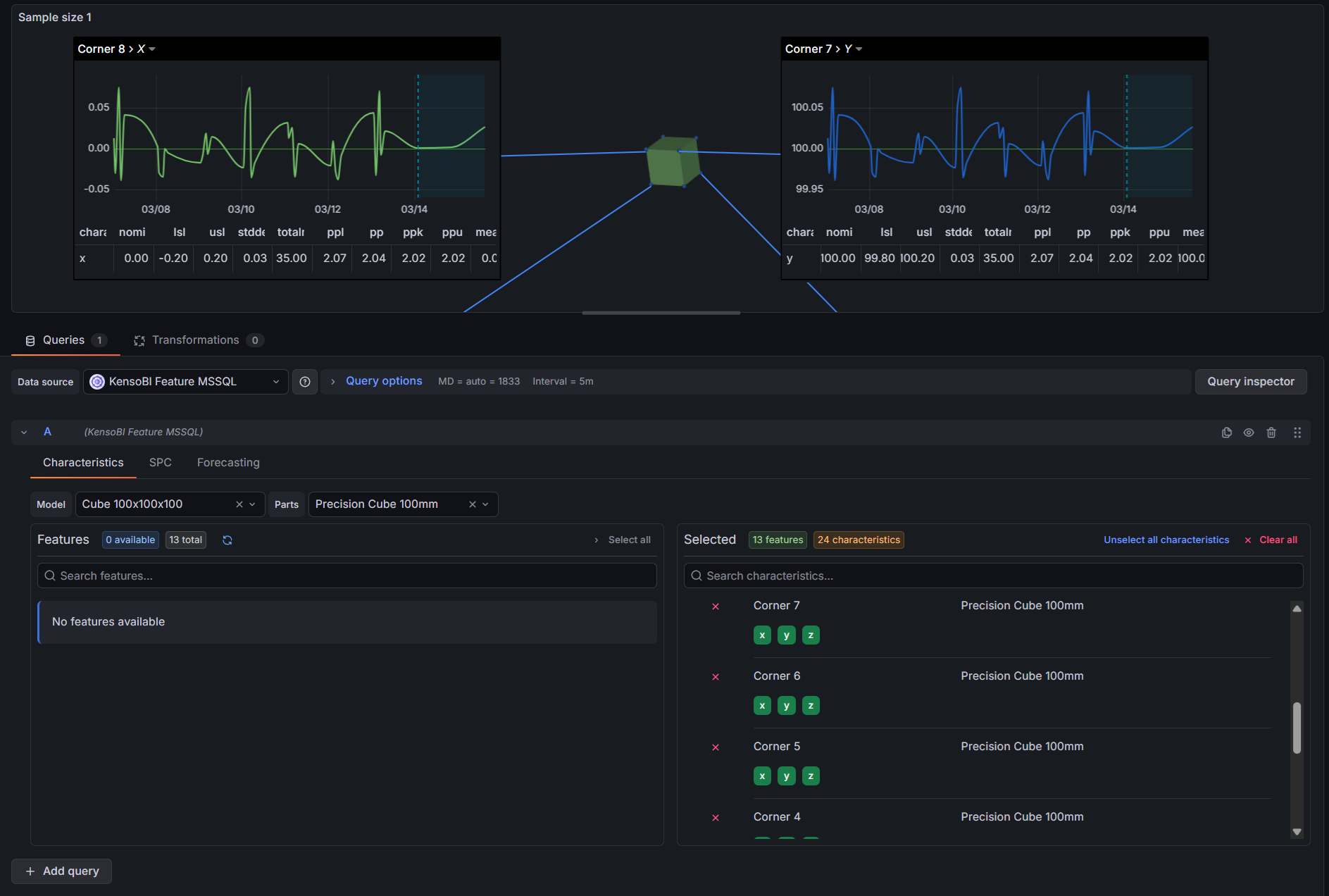
Table of Contents

• Why SPC Characteristic Datasource?
• Features
• Use Cases
• Requirements
• Getting Started
• Configuration
  • Database Connection
  • Schema Mapping
  • Preset Schemas
  • Custom Schema Mapping
• Query Editor
  • Characteristics Tab
  • SPC Tab
  • Forecasting Tab
• SPC Calculations
  • Sample Size and Aggregation Type
  • Available Statistics
  • Control Limits
  • Capability Indices
• Forecasting
  • Moving Average
  • Linear Regression
  • Holt (Double Exponential Smoothing)
  • Holt-Winters (Triple Exponential Smoothing)
  • Confidence Bands
• Output Frames
• Part of the KensoBI SPC Suite
• Getting Help
• License

---

Why SPC Characteristic Datasource?

The SPC CAD Panel displays CAD models in 3D with clickable feature annotations. Each annotation can show measurement tables, embedded trend charts, and forecast lines — but it needs a datasource that understands the structure of a measurement database and returns data in the right shape.

That is what this datasource does. It connects to your PostgreSQL or MSSQL measurement database, gives you a point-and-click interface to select which features and characteristics to include, and returns everything the CAD panel needs in a single query:

• features frame — one row per characteristic with SPC statistics (mean, UCL/LCL, Cp/Cpk, etc.) and metadata (nominal, LSL, USL). This is what populates the annotation tables and drives the color-coding rules in the CAD panel.
• timeseries frame — individual measurements over time for each characteristic. This is what the CAD panel's embedded trend charts and SPC chart components display.
• forecast-upper-bound / forecast-lower-bound frames — predicted future values with confidence intervals. The CAD panel renders these as a forecast line with a shaded confidence band extending beyond the last measurement.

Writing this SQL by hand for every characteristic on every dashboard would be impractical. The SPC Characteristic Datasource builds and executes the correct nested subgroup aggregation queries automatically, applying the right Shewhart constants for your sample size and chart type.

Features

Feature	Description
Visual feature selector	Transfer-list UI to browse and select features and characteristics by model and part
Cascading filters	Selecting a model narrows the parts list; selecting a part narrows the features list
SPC statistics	Mean, UCL/LCL, Cp, Cpk, CPL, CPU, Cpm, Pp, Ppk, std dev, min, max, total in tolerance, and more
Subgroup aggregation	Configurable sample size (1–10) with mean, range, or standard deviation aggregation type
Time series output	Individual measurements over time, one column per characteristic
Built-in forecasting	Moving Average, Linear Regression, Holt, and Holt-Winters — runs in the browser, no external service
Forecast confidence bands	Upper and lower prediction intervals at 80%, 90%, 95%, or 99% confidence
Schema presets	One-click setup for KensoBI and Q-DAS database schemas
Custom schema mapping	Map any database structure with table and column pickers
Custom columns	Add extra columns from any mapped table to the output frames
PostgreSQL and MSSQL	Delegates query execution to any existing Grafana SQL datasource

Use Cases

• Interactive CAD inspection reports — bind measurements to 3D part geometry in the SPC CAD Panel; click any feature to see its statistics, trend chart, and forecast
• Process capability monitoring — track Cp, Cpk, Pp, and Ppk per characteristic directly in annotation tables
• Early warning forecasting — detect when a characteristic is trending toward a specification limit before it gets there
• Q-DAS database integration — connect directly to existing QDAS measurement databases without modifying the schema
• Custom metrology databases — map any database that follows the feature → characteristic → measurement pattern

Requirements

• Grafana 11.6.10 or later
• A configured Grafana PostgreSQL or MSSQL datasource pointing to your measurement database

---

Getting Started

1. Install the SPC Characteristic Datasource from the Grafana Plugin Catalog.
2. In Grafana, go to Administration → Data sources → Add new data source and search for SPC Characteristic.
3. Under Database Connection, select the existing PostgreSQL or MSSQL datasource that connects to your measurement database.
4. Under Schema Mapping, click Kenso Preset or QDAS Preset if your database uses one of those schemas, or configure the table and column mappings manually.
5. Click Save & test to verify the connection.
6. Open an SPC CAD panel, set the data source to SPC Characteristic, and open the query editor.
7. In the Characteristics tab, filter by model or part, then move features to the right-hand list.
8. Open the SPC tab to enable the statistics you want in annotation tables (mean, UCL/LCL, Cp/Cpk, etc.).
9. Optionally open the Forecasting tab to enable forecast lines in annotation trend charts.

---

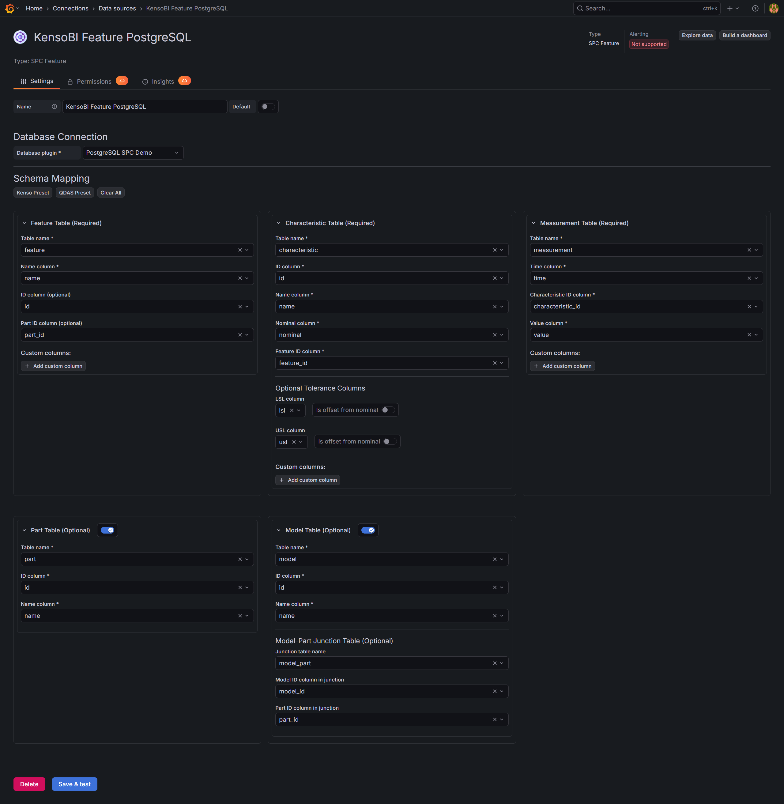
Configuration

Database Connection

The SPC Characteristic Datasource does not connect directly to your database. Instead, it delegates query execution to an existing Grafana SQL datasource. Connection credentials, SSL settings, and authentication are all managed by the underlying SQL datasource — the SPC Characteristic Datasource only adds the query-building and SPC calculation layer on top.

Supported underlying datasource types:

Plugin	Type identifier
Grafana PostgreSQL	grafana-postgresql-datasource
Grafana MSSQL	grafana-mssql-datasource
MSSQL (legacy)	mssql

Select the database plugin from the Database plugin dropdown. Only datasources of the supported types will appear.

Schema Mapping

After selecting a database plugin, configure the Schema Mapping section. This tells the datasource which tables and columns hold your feature, characteristic, and measurement data.

The schema is split into three required sections and two optional sections:

Section	Required	Description
Feature Table	Yes	The table listing geometric features (holes, surfaces, edges, etc.)
Characteristic Table	Yes	The table listing measurable characteristics with nominal values and tolerances
Measurement Table	Yes	The table containing individual measurement records with timestamps
Part Table	No	Enables filtering features by part name in the query editor
Model Table	No	Enables filtering parts by model and enables the Model dropdown in the query editor

Each section uses dropdown pickers populated by automatic schema discovery from your database connection, so you can point and click rather than type names.

Preset Schemas

Click one of the preset buttons to populate all required fields automatically:

Kenso Preset — matches the KensoBI measurement database schema:

Table	Columns	Purpose
feature	id, name, part_id	Feature identifier and name
characteristic	id, name, nominal, feature_id, lsl, usl	Characteristic with tolerance offsets from nominal
measurement	time, characteristic_id, value	Individual measurements
part	id, name	Parts
model	id, name via model_part junction	Models

Note: In the Kenso schema, lsl and usl are stored as offsets from nominal (LSL = nominal + lsl, USL = nominal + usl).

QDAS Preset — maps to the Q-DAS merkmal/wertevar schema commonly used by CMM software:

Table	Columns	Purpose
merkmal	memerkmal, memerknr, menennmas, meugw, meogw	Characteristics (features extracted from memerknr pattern)
wertevar	wvdatzeit, wvmerkmal, wvwert	Individual measurements
teil	teteil, tebezeich	Parts

Note: QDAS does not support a model table. Tolerances are also stored as offsets from nominal.

Custom Schema Mapping

If your database uses a different structure, configure each section manually:

Feature Table

Field	Required	Description
Table name	Yes	Name of the feature table
Name column	Yes	Column containing the feature display name
ID column	No	Primary key column. If omitted, the name column is used as the ID
Part ID column	No	Foreign key to the part table — required for part-based filtering
Custom columns	No	Additional columns to include in the output features frame

Characteristic Table

Field	Required	Description
Table name	Yes	Name of the characteristic table
ID column	Yes	Unique identifier for each characteristic
Name column	Yes	Display name shown in the query editor and output
Nominal column	Yes	Reference/target value for the characteristic
Feature ID column	Yes	Foreign key to the feature table
LSL column	No	Lower specification limit column
LSL is offset	No	If enabled, actual LSL = nominal + column value
USL column	No	Upper specification limit column
USL is offset	No	If enabled, actual USL = nominal + column value
Custom columns	No	Additional columns to include in the output features frame

Measurement Table

Field	Required	Description
Table name	Yes	Name of the measurement table
Time column	Yes	Timestamp column — used for $__timeFilter and time series output
Characteristic ID column	Yes	Foreign key to the characteristic table
Value column	Yes	Numeric measurement value
Custom columns	No	Additional columns to include in the time series output

Model Table (optional)

When enabled, you can also configure a junction table for the model-to-part relationship if your schema uses a separate join table (e.g., model_part).

---

Query Editor

The query editor has three tabs: Characteristics, SPC, and Forecasting.

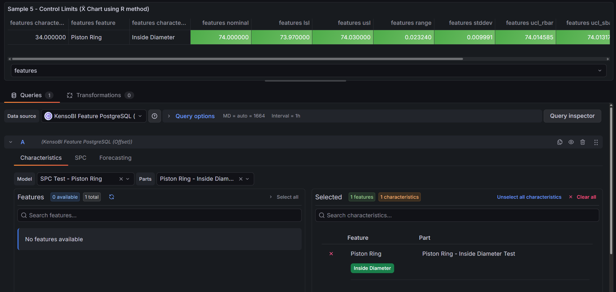
Characteristics Tab

The Characteristics tab is where you choose which data to query.

Filters:

• Model — filters the parts list to only parts belonging to the selected model. Only shown when the Model Table is configured in the datasource settings.
• Parts — filters the features list to only features belonging to the selected part. Selecting a model automatically narrows the available parts.

Transfer list:

The left side shows all available features for the selected model/part combination. Click a feature to move it to the right side (selected). Click it again to deselect it.

When you select a feature, all of its characteristics are added automatically. Below each selected feature on the right side, the individual characteristics are listed as toggle buttons. Characteristics are enabled by default — click one to exclude it from the query. Excluding a characteristic removes it from both the features and timeseries frames, which reduces the amount of data the CAD panel needs to process.

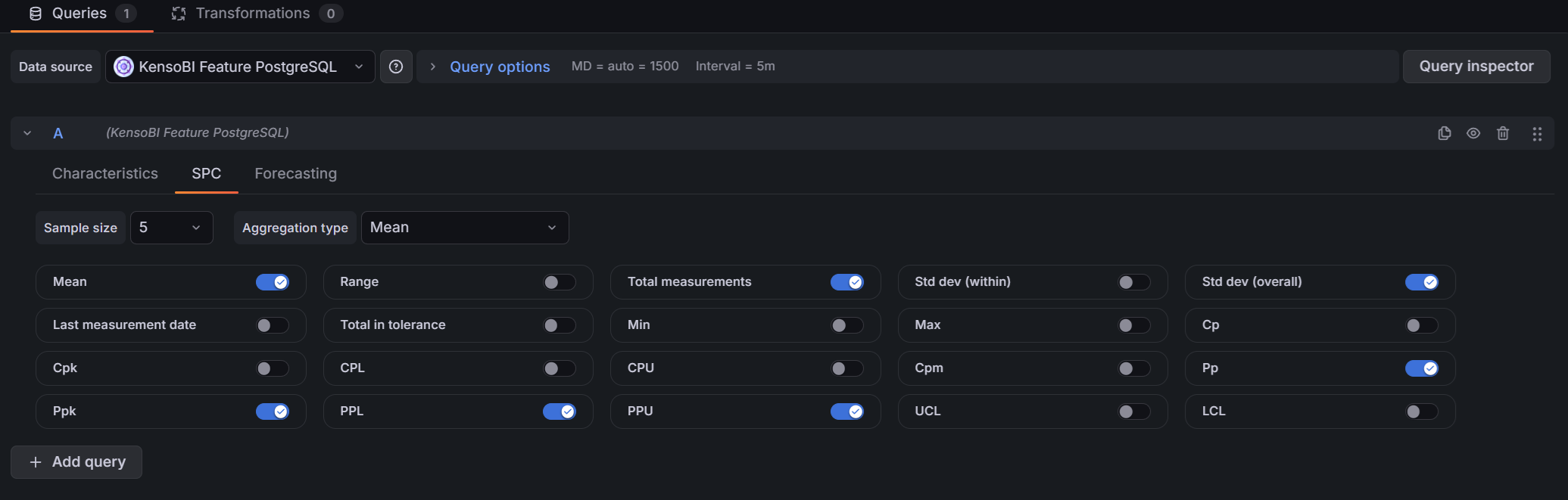
SPC Tab

The SPC tab controls which statistics are included in the features frame — the frame that populates annotation tables and drives color-coding rules in the SPC CAD panel.

Top controls:

Control	Description
Sample size	Number of consecutive measurements to group into one subgroup (1–10). Size 1 returns individual measurement statistics with no subgroup aggregation.
Aggregation type	How each subgroup is summarized. Only shown when sample size > 1. Options: Mean (X̄-R or X̄-S chart), Range (R-chart), Standard deviation (S-chart).

Available statistics (toggles):

Statistic	Description	Availability
Mean	Grand mean of all measurements (X̄̄)	Always
Range	Global range (max − min of all measurements)	Always
Total measurements	Count of all measurements in the time range	Always
Std dev (within)	Within-subgroup standard deviation estimate (σ̂ = R̄/d₂ or S̄/c₄)	Sample size > 1 only
Std dev (overall)	Long-term standard deviation of all individual measurements	Always
Last measurement date	Timestamp of the most recent measurement	Always
Total in tolerance	Count of measurements within [LSL, USL]	Always
Min	Minimum subgroup aggregate (or minimum measurement if n=1)	Always
Max	Maximum subgroup aggregate (or maximum measurement if n=1)	Always
Cp	Short-term potential capability index	Sample size > 1, Mean aggregation only
Cpk	Short-term centered capability index	Sample size > 1, Mean aggregation only
CPL	Lower capability index: (mean − LSL) / 3σ̂	Sample size > 1, Mean aggregation only
CPU	Upper capability index: (USL − mean) / 3σ̂	Sample size > 1, Mean aggregation only
Cpm	Taguchi capability index	Sample size > 1, Mean aggregation only
Pp	Long-term performance capability index	Mean aggregation only
Ppk	Long-term centered performance capability index	Mean aggregation only
PPL	Lower performance index: (mean − LSL) / 3σ	Mean aggregation only
PPU	Upper performance index: (USL − mean) / 3σ	Mean aggregation only
UCL	Upper Control Limit	Sample size > 1 only
LCL	Lower Control Limit	Sample size > 1 only

Forecasting Tab

The Forecasting tab adds a forecast to the query response. When a model is selected, the datasource appends forecast-upper-bound and forecast-lower-bound frames alongside the standard timeseries frame. The SPC CAD Panel uses these frames to draw a forecast line with a shaded confidence band in annotation trend charts, extending beyond the last measured value.

Model selection:

Model	Best for
Disabled	No forecasting (default)
Moving Average	Stable data with no trend
Linear Regression	Data with a clear linear trend
Holt (Trend)	Evolving trends without seasonality
Holt-Winters (Seasonal)	Data with repeating seasonal patterns

Common parameters:

Parameter	Description	Default
Forecast Periods	Number of future time steps to project	10
Confidence Level	Width of the prediction interval: 80%, 90%, 95%, or 99%	95%

Moving Average parameters:

Parameter	Description	Default
Window Size	Number of recent measurements to average per step	5

Holt parameters:

Parameter	Description	Default
Alpha (Level)	Smoothing factor for the level component (0–1)	0.5
Beta (Trend)	Smoothing factor for the trend component (0–1)	0.5
Phi (Damping)	Trend damping factor (0–1]. 1.0 = linear extrapolation; 0.9 = trend decays over time	0.9

Holt-Winters parameters:

Parameter	Description	Default
Alpha (Level)	Smoothing factor for the level component (0–1)	0.5
Beta (Trend)	Smoothing factor for the trend component (0–1)	0.5
Phi (Damping)	Trend damping factor (0–1]. 1.0 = linear extrapolation; 0.9 = trend decays over time	0.9
Gamma (Seasonal)	Smoothing factor for the seasonal component (0–1)	0.5
Season Length	Number of periods in one season (e.g., 24 for hourly data with a daily pattern)	24

caution

Holt-Winters requires at least 2 complete seasons of data. For example, with Season Length = 24 you need at least 48 data points. If no forecast appears, reduce the season length or extend the dashboard time range to include more historical data.

Quick Presets:

Preset	Model	Periods	Notes
+12h Moving Average	Moving Average	6	Window size 5
+24h Linear Trend	Linear Regression	12	—
+2d Holt (Trend)	Holt	24	α=0.5, β=0.5, φ=0.9
+1w Holt-Winters (Daily)	Holt-Winters	168	Season 24, hourly data

---

SPC Calculations

Sample Size and Aggregation Type

The datasource uses a three-level nested SQL query to compute SPC statistics:

1. Inner query — selects individual measurement rows within the dashboard time range and assigns each row a sequential sampleNumber based on sample size
2. Middle query — groups by sampleNumber and characteristic_id to compute the subgroup aggregate (sampleAgg): mean, range, or standard deviation per subgroup
3. Outer query — aggregates across all subgroups to produce the final statistics returned in the features frame

When sample size = 1, the three-level structure simplifies: no subgroup grouping is performed and the statistics describe the population of individual measurements directly.

Available Statistics

Output column	Formula (mean aggregation)
mean	avg(sampleAgg) — grand mean of subgroup means
range	max(value) - min(value) — range of all individual measurements
totalMeasurements	count(value)
standardDeviation (within)	avg(sampleRange) / d₂ (R-chart) or avg(sampleStdDev) / c₄ (S-chart)
stdDevOverall	stddev_pop of all individual measurements, reconstructed from sum/sumSq/count
lastMeasurementDate	max(time)
totalInTolerance	Count of measurements where LSL ≤ value ≤ USL
min	min(sampleAgg) — minimum subgroup mean (or min measurement if n=1)
max	max(sampleAgg) — maximum subgroup mean (or max measurement if n=1)

Control Limits

Control limits are computed using Shewhart constants injected as Grafana template variables. The appropriate formula depends on the aggregation type:

X̄ chart (mean aggregation):

Limit	Formula
UCL (rbar)	X̄̄ + A₂ × R̄
UCL (sbar)	X̄̄ + A₃ × S̄
LCL (rbar)	X̄̄ − A₂ × R̄
LCL (sbar)	X̄̄ − A₃ × S̄

Both variants are returned when mean aggregation is selected — use ucl_rbar/lcl_rbar for X̄-R charts, or ucl_sbar/lcl_sbar for X̄-S charts.

R chart (range aggregation):

Limit	Formula
UCL	D₄ × R̄
LCL	D₃ × R̄

S chart (standard deviation aggregation):

Limit	Formula
UCL	B₄ × S̄
LCL	B₃ × S̄

The Shewhart constants (A₂, A₃, B₃, B₄, D₃, D₄, d₂, c₄) are automatically selected based on the configured sample size. They cover sample sizes 2 through 10.

Capability Indices

Capability indices are only available when sample size > 1 and aggregation type = Mean. They require LSL and/or USL to be configured in the characteristic table schema mapping.

Index	Formula	Notes
Cp	(USL − LSL) / (6σ̂)	Both LSL and USL required
Cpk	min((USL − μ) / 3σ̂, (μ − LSL) / 3σ̂)	One limit sufficient
CPL	(μ − LSL) / 3σ̂	Lower short-term index
CPU	(USL − μ) / 3σ̂	Upper short-term index
Cpm	(USL − LSL) / (6 × √(σ̂² + (μ − T)²))	Taguchi index; T = nominal
Pp	(USL − LSL) / (6σ)	Both limits required
Ppk	min((USL − μ) / 3σ, (μ − LSL) / 3σ)	One limit sufficient
PPL	(μ − LSL) / 3σ	Lower long-term index
PPU	(USL − μ) / 3σ	Upper long-term index

Notation:

• μ = grand mean (X̄̄)
• σ̂ = within-subgroup standard deviation estimate (R̄/d₂ or S̄/c₄)
• σ = overall standard deviation (stddev_pop of all individual measurements)

Interpretation:

Value	Interpretation
Cp/Cpk < 1.00	Not capable — producing output outside specification
1.00 ≤ Cp/Cpk < 1.33	Marginally capable
1.33 ≤ Cp/Cpk < 1.67	Capable — meets most industry requirements
Cp/Cpk ≥ 1.67	Highly capable

A large gap between Cp and Cpk means the process is capable in potential but poorly centered.

---

Forecasting

All forecast algorithms run entirely in the browser — no external service or API call is required. The datasource computes forecast values after the historical measurement data is returned from the database.

Moving Average

Projects the last windowSize measurement values forward. Each forecast step is the average of the most recent window.

$\hat{y}_{t+h} = \frac{1}{w} \sum_{i=t-w+1}^{t} y_i$

Best for: Flat, stable processes with no visible trend or seasonality.

Linear Regression

Fits an ordinary least-squares line to the full measurement history and extrapolates it forward. The confidence interval uses a t-distribution with n−2 degrees of freedom.

$\hat{y} = a + b \cdot t$

Best for: Processes with a clear, consistent linear drift (e.g., tool wear).

Holt (Double Exponential Smoothing)

Tracks both the level and trend using separate smoothing factors. The optional damping factor (φ) causes the trend to decay toward zero over the forecast horizon, preventing unrealistic long-range extrapolation.

$\hat{y}_{t+h} = \ell_t + (\phi + \phi^2 + \cdots + \phi^h) \cdot b_t$

Parameter	Effect
Alpha (α)	Higher = faster response to level changes; lower = smoother
Beta (β)	Higher = faster response to trend changes
Phi (φ)	1.0 = linear trend (no damping); 0.9 = trend fades out over time

Best for: Evolving trends where you want to temper long-range predictions with damping.

Holt-Winters (Triple Exponential Smoothing)

Extends Holt's method with a seasonal component. Handles additive seasonality (repeating patterns of fixed magnitude). Requires at least two complete seasons of historical data.

$\hat{y}_{t+h} = (\ell_t + b_t \cdot h) + s_{t+h-m}$

Parameter	Effect
Alpha (α)	Level smoothing
Beta (β)	Trend smoothing
Phi (φ)	Trend damping
Gamma (γ)	Seasonal smoothing — how quickly seasonal patterns adapt
Season Length	Number of periods per season (e.g., 24 for hourly data with a daily cycle)

Best for: Processes that follow a known periodic cycle — daily production patterns, weekly shifts.

Confidence Bands

The datasource outputs upper and lower confidence bound frames for each forecast model:

Level	z-score
80%	1.282
90%	1.645
95%	1.960
99%	2.576

Linear regression uses a t-distribution instead of z-scores when the sample size is small. The interval widens as the forecast horizon increases to reflect growing uncertainty. The SPC CAD Panel renders these bounds as a shaded confidence band around the forecast line.

---

Output Frames

Each query returns up to four Grafana data frames. The SPC CAD Panel identifies each frame by its name property (stored in meta.custom.frameType):

Frame name	frameType	Used by SPC CAD for
features	features	Annotation tables, color-coding rules, nominal/LSL/USL values
timeseries	timeseries	Embedded trend charts and SPC chart components in annotations
forecast-upper-bound	forecast-upper-bound	Upper edge of the confidence band in annotation trend charts
forecast-lower-bound	forecast-lower-bound	Lower edge of the confidence band in annotation trend charts

features frame columns:

Always present:

• characteristic_id — unique characteristic identifier
• characteristic_name — display name
• feature — feature name
• nominal — nominal value
• lsl — lower specification limit (if configured)
• usl — upper specification limit (if configured)

Plus any selected SPC statistics (mean, ucl, lcl, cp, cpk, etc.) and any custom columns defined in the schema mapping.

timeseries frame columns:

• time — measurement timestamp
• One column per selected characteristic (named by characteristic_id) containing the measured value

forecast-* frame columns:

• time — forecast timestamp (future)
• One column per characteristic with the forecasted value

note

The features and timeseries frames are always produced when characteristics are selected. The forecast-upper-bound and forecast-lower-bound frames are only added when a forecast model is configured in the Forecasting tab.

---

Part of the KensoBI SPC Suite

SPC CAD Panel — the primary consumer of this datasource. Displays CAD models in 3D with interactive feature annotations driven by the features, timeseries, and forecast frames this datasource produces.

SPC Chart Panel — control charts (XmR, Xbar-R, Xbar-S) for monitoring process stability over time.

SPC Histogram Panel — distribution analysis with histograms, bell curves, and a statistics table showing Cp, Cpk, Pp, and Ppk.

SPC Box Plot Panel — box-and-whisker plots with Xf-Rf resistant control limits.

SPC Bullet Panel — compact bullet charts and progress bars with optional SPC metrics (Cpk, Cp, Ppk, Pp, Sigma Level) computed from the full time series. Use it to build dense KPI dashboards that show process capability at a glance.

SPC Pareto Panel — Pareto charts for identifying the most significant defect sources.

---

Getting Help

• Contact support at https://kensobi.com/contact
• Join the KensoBI Discord for questions and discussion.

License

This software is distributed under the Kenso Software Commercial License. Use requires a valid commercial license.